All published articles of this journal are available on ScienceDirect.

High Accuracy Diagnosis for MRI Imaging Of Alzheimer’s Disease using Xgboost
Abstract
Introduction:
Alzheimer’s disease (AD) is the most epidemic type of dementia. The cause and treatment of the disease remain unidentified. However, when the impairment is still at a preliminary stage or mild cognitive impairment (MCI), the symptoms might be more controlled, and the treatment can be more efficient. As a result, computational diagnosis of the disease based on brain medical images is crucial for early diagnosis.
Methods:
In this study, an efficient computational method was introduced to classify MRI brain scans for patients with Alzheimer’s disease (AD), mild cognitive impairment (MCI), and normal aging control (NC), comprising three main steps: I) feature extraction, II) feature selection III) classification. Although most of the current approaches utilize binary classification, the proposed model can differentiate between multiple stages of Alzheimer’s disease and achieve superior results in early-stage AD diagnosis. 158 magnetic resonance images (MRI) were taken from the Alzheimer’s Disease Neuroimaging Initiative database (ADNI), which were preprocessed and normalized to be suitable for extracting the volume, cortical thickness, sulci depth, and gyrification index measures for various brain regions of interest (ROIs), as they play a considerable role in the detection of AD. One of the embedded feature selection method was used to select the most informative features for AD diagnosis. Three models were used to classify AD based on the selected features: an extreme gradient boosting (XGBoost), support vector machine (SVM), and K-nearest neighborhood (KNN).
Results and Discussion:
XGBoost showed the highest accuracy of 92.31%, precision of 0.92, recall of 0.92, F1-score of 0.92, and AUC of 0.9543. Recent research has reported using multivariable data analysis to classify dementia stages such as MCI and AD and employing machine learning to predict dementia stages.
Conclusion:
In the proposed method, we achieved good performance for early-stage AD (MCI) detection, which is the most targeted stage to be identified. Moreover, we investigated the most reliable features for the diagnosis of AD.
1. INTRODUCTION
Alzheimer's disease (AD) is a cumulative neurodegenerative disease for which there is currently no cure. However, the detection of the disease at an earlier stage can assist in slowing down the progression of AD. Neuropathological changes due to AD appear prior to the onset of clinical symptoms. Hence, there is a need to detect brain alterations at an early stage and identify biomarkers that are most associated with mild cognitive impairment (MCI) and AD.
Structural magnetic resonance images (MRI) biomarkers, including brain regions morphometry, texture, volume, and cortical measurements, have been used to classify the main stages of Alzheimer’s disease: normal control (NC), MCI, and AD. Many automatic approaches have been used for extracting biomarkers from MRI [1-5], such as region of interest analysis (ROI) methods. ROI analysis aims to map labeled ROIs from a brain atlas (volume and surface-based atlas maps) to a target brain via automated high-dimensional registration to obtain labeled ROIs from the target. Following this, regional tissue measurements such as ROI volume, cortical thickness, sulcal depth, and gyrification index were estimated. To accomplish this automatic feature extraction and analysis, there are various software packages such as Statistical Parametric Mapping (SPM), Computational Anatomy Toolbox (CAT12) [6], and FreeSurfer [7].
The chief concern addressed in several studies for diagnosing AD at its early stages are building more efficient biomarkers from MRI scans for AD detection. The use of various machine learning classifiers to select features related to Alzheimer's and to develop an accurate detection system is a current area of research. MRI scans have been studied to obtain several Alzheimer's biomarkers and to study the most atrophic regions using volume [8, 9], shape [10], texture [11], cortical [12, 13], and sulcal measurements [14]. These measurements were performed on various affected brain regions, including the hippocampus [15], amygdala [16, 17], whole brain [18], entorhinal cortex [19], brainstem [20] and ventricles [21]. Although volume and cortical thickness are the most dominant biomarkers studied, there have been very few investigations of other surface-based features, such as the gyrification index and sulcal depth in early AD diagnosis. Analysis of the gyrification index and sulcal depth could provide remarkable information about the alterations in the brain shape caused by AD. These alterations are not detected with conventional volumetric analyses but could be captured with cortical gyrification analysis [22]. The sulcal depth and sulcal width were observed to be lower in normal controls and increasing along with the severity level of AD [12, 14]. The gyrification index, which is the ratio of the inner surface (GM/WM interface) area to the outer surface area (GM/CSF interface), is an excellent feature for the early diagnosis of patients with mild AD and for separating them from normal controls [22]. Some researchers believed combining complementary biomarkers with different information could provide more efficient and accurate evidence for AD, MCI, and NC diagnosis [23].
Recent advances in machine learning techniques, such as support vector machine (SVM), K-nearest neighbor (KNN), decision tree [24], and ensemble models [25], enhance the process of disease diagnosis and increase the accuracy through automated systems instead of focusing entirely on physician experiments. However, selecting the best biomarkers that represent Alzheimer's is a major challenge that can be used to distinguish between stages of the disease. The particle swarm optimization (PSO) algorithm [26], XGBoost [27], RFE-SVM [28], and t-test [29] are some of the feature selection methods that have been employed in recent studies. One study developed a method by combining SVM and particle swarm optimization (PSO) for classifying AD from NC with an accuracy of up to 94.12% and 88.89% for classifying MCI from NC, using volume and shape features [30]. Another study demonstrated 96.5% classification accuracy for AD/NC by investigating the temporal lobe and whole-brain gray matter [31]. Furthermore, a multistage classifier-based method used 88 features (50 volumes and 38 regional cortical thicknesses) to predict AD/MCI/NC with an accuracy of up to 81.3%. On the other hand, one report obtained 0.52 average precision and 0.56 average recall for classifying AD, MCI and NC using an ensemble random forest. Moreover, a surface-based morphometry report differentiated between AD and NC with 93.3% specificity and 87.1% sensitivity [32].
Our contribution is to have the most beneficial number of features among a large pool of AD biomarkers to differentiate between AD stages and diagnose the early stage with high accuracy using XGBoost. In this study, MRI scans were acquired from the Alzheimer’s Disease Neuroimaging Initiative (ADNI) and processed to extract volumetric features for 81 brain regions. In addition, cortical thickness, sulcal depth, and gyrification index features were obtained for 68 brain regions, and all features were combined to get 275 attributes. We used XGBoost to find the best features that represent Alzheimer's disease in order to build a more precise classification system. At last, three different classifiers (XGBoost, SVM, and KNN) were used to compare the classification accuracies.
2. MATERIALS AND METHODS
2.1. Database
Data required for this study were obtained from the Alzheimer's Disease Neuroimaging Initiative (ADNI) database (http://adni.loni.usc.edu). ADNI was propelled as a public-private corporation by six nonprofit organizations in 2003: the National Institute on Aging (NIA), the National Institute of Biomedical Imaging and Bioengineering (NIBIB), the Food and Drug Administration (FDA), and private pharmaceutical companies. ADNI's main objective was to check whether specific biomarkers, clinical and neuropsychological assessment, positron emission tomography (PET), and serial MRI can be combined to evaluate MCI evolution and early Alzheimer's.
158 T1-weighted MRI scans have been taken from ADNI, 26 female cases and 28 male cases in AD stage, 28 females and 25 males in NC stage and in MCI stage, 27 females and 24 males. The age range of the participants was 50-85 years. The imaging parameters were as follows: magnetic field strength =3T, flip angle= 9°, repetition time = 2,300 ms, echo time = 3.0 ms, slice thickness =1.2 mm, acquisition matrix = 240 ×256, pixel spacing X=1.0 mm; pixel spacing Y=1.0 mm and number of slices = 176. Some criteria were not considered in the dataset, such as the Clinical Dementia Rating Scale (CDR), Mini-Mental State Examination (MMSE), chronic diseases and medical history of the patient. The demographic characteristics of the subjects are presented in Table 1.
| Class | Female | Male | Sample Size/Each Class |
|---|---|---|---|
| AD | 26 | 28 | 54 |
| MCI | 27 | 24 | 51 |
| NC | 28 | 25 | 53 |
| Total | 81 | 77 | 158 |
2.2. Image Analysis
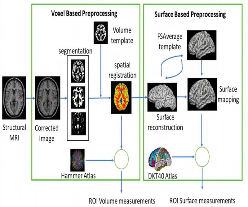
Data were collected from ADNI and preprocessed using CAT12. The preprocessing workflow included a spatial adaptive nonlocal means (SANLM) denoising filter [33] to reduce noise while preserving edges, bias field inhomogeneity correction, and affine registration to get further high-quality segmentation outcome, skull stripping with adaptive probability region growing (APRG) approach, and segmentation to three tissues (GM, WM and CSF) using Adaptive Maximum A Posterior (AMAP) technique [34]. After that, spatial normalization of the three tissues was performed using the DARTEL [35] template. Then, the Hammers atlas [36], one of the volume atlases, was used to calculate GM and WM volumes for specific brain regions. Surface-based processing was performed following the completion of the previous processing. The projection-based thickness (PBT) method [37] estimated cortical thickness, and the central cortical surface was reconstructed. The central surface is the surface between the inner (WM/GM boundary) and outer (GM/CSF boundary) cortical surfaces, which represent the cortex well, and enable reliable estimation of cortical parameters (GI, SD). Ultimately, 71 raw volumetric measurements and 68 cortical thickness (CT), 68 gyrification indexe (GI), and and measurements 68 sulcal depth (SD) measurements were extracted. Volume measurements involving the hippocampus, amygdala, temporal pole, fusiform, insula, putamen, thalamus, lateral temporal ventricle, and cuneus were normalized by the intracranial volume. Relative volumes provided more precise volumes by reducing the influence of factors such as head size and brain size. Surface-based features (CT, GI, and SD) include entorhinal, temporal pole, insula, fusiform, parahippocampus, insula, etc. By combining volume with surface-based features, we will collect most of the important parameters to indicate the existence of the disease, as they are complementary biomarkers with valid information (Fig. 1).
2.3. Features Selection
The feature selection process uses a specific algorithm to determine the most dominant features contributing more to the prediction variable to improve model accuracy and reduce computational cost. There are three feature selection methods: filter, wrapper, and embedded. In embedded methods, feature selection can be used as a part of the training process, as the model picks features that maximize accuracy [38]. Embedded methods have an advantage over wrapper methods because they eliminate the computation time required to reclassify different subsets. Moreover, they outrank filter methods by considering the dependencies between features [39]. Therefore, there is no need to take the step of inspecting the correlation between features. Thus, we used one of the embedded feature selection methods, XGBoost, to get the top-ranked features.
We have a high-dimensional feature vector, 68×3 surface-based features (cortical thickness, sulcal depth, gyrification index), and 71 volumetric features, and not all have important information for diagnosing AD.
In XGBoost, we chose the gain value associated with each feature to rank them. The gain parameter for each feature corresponds to the average loss reduction gained when using this feature to split trees. After feature ranking, we built a model by progressively increasing the feature size, starting with the most important features and recording the accuracy. The accuracy stabilized from Features 16 to 21. From Feature 21, it decreased by 15% approximately. Adding more features will not improve the performance and will make the model more complex. Thus, the number of features is limited to 16.
2.4. Classification
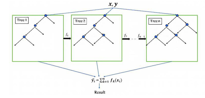
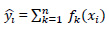
In the classification step, two conventional techniques have been used: SVM, KNN, and one of the recent technology models, such as XGBoost. XGBoost is an enhanced version of the gradient boosting ensemble learning method with highly precise and promising results, which is implemented by Guestrin [40]. XGBoost comprises a series of decision trees (weak learners) that are created in a sequential manner and consequently combine their decisions to predict the target. As shown in Fig. (2), one tree (weak classifier) is fitted to a split of features to begin the training. It then fits another tree based on the training error (residual) from the previous tree, and this process is repeated. The final predicted output combines all results of the tree.
The prediction function is defined as:
 |
(1) |
Where yi is the predicted class of the i-th observation, xi is the corresponding feature vector, and k is the total number of decision trees ƒk(xi) defined as:
 |
(2) |
wqk(xi) is the structure-function of the k-th decision tree that maps xi to the corresponding leaf node, w is the vector of leaf weights.
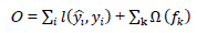
XGBoost uses gradient descent to minimize the errors of weak learners. The objective function is expressed as follows:
 |
(3) |
where  is the loss function that measures the deviation between the prediction
  and the true value yi,
  is the regularization term. (Tree model complexity penalty term) Ω(ƒk) is defined as:
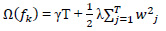 |
(4) |
where T is the number of leaf nodes, γ is the weight of the leaf nodes, and λ and w are regular coefficients. The model is being trained in an additive manner. Let  be the predicted value of the i-th observation at the t-th iteration, and the prediction function is:
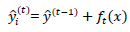 |
(5) |
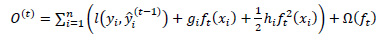
And the objective function is altered to:
 |
(6) |
The regularization function is responsible for stopping the training of a model when the function determines that the model is sufficiently effective based on the learning score, thereby avoiding the risk of overfitting.
XGBoost uses the second Taylor approximation to optimize the objective function quickly.
 |
(7) |
XGBoost is faster than gradient boosting because it uses the power of parallel processing, which makes it possible to train on large data in a better manner. It also deals with small and sparse data efficiently and uses regularization to avoid overfitting. XGBoost includes a large variety of tuning parameters for cross-validation, regularization, user-defined objective functions, missing values, and tree parameters. It uses the features of each MRI image to train and evaluate the importance score, which implies how significant the related feature was in buildingthe boosted decision trees within the model. The values used for each parameter are explained in Table 2.
| Parameter | Default | Description |
|---|---|---|
| Learning rate (eta) | 0.3 | Shrink the weights on each step |
| N_estimators | 100 | Number of trees to fit in our ensemble. |
| Objective | multi: softprob | Softprob is the same as softmax objective, for multiclassification |
| Booster | gbtree | Select the model for each iteration |
| Nthread | max | The core number in the system, used for parallel processing |
| Minchildweight | 1 | Minimum sum of weights |
| Max_depth | 3 | Maximum depth of a tree. |
| Gamma(γ) | 0 | The minimum loss reduction needed for splitting |
| Subsample | 1 | Control the sample’s proportion |
| Colsample_bytree | 1 | Column’s fraction of random samples |
| Reg_lambda(λ) | 1 | L2 regularization term on weights |
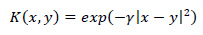
SVM is a supervised machine learning model used for classification or regression and has been broadly used in various successful applications. SVM chooses the best hyper-plane or a group of hyper-planes that maximizes the distance of the margin between classes to classify data. For non-linearly separable data, SVM utilizes a kernel function that maps the input data (training samples) to a higher dimensional space, such as Gaussian kernel [41]:
 |
(8) |
Where γ is gamma, which controls the influence of each training point has on the position of the decision boundary, |x – y|2 can be defined as squared the Euclidean distance between the two feature vectors.
We used a polynomial kernel, and the polynomial order was 3 and the box constraint was 5.23.
KNN is a supervised nonparametric machine learning method. It stores and arranges all labeled data in memory during the training process; therefore, it is memory dependent and does not require model fitting. The test point is then classified based on a similarity measure between this point and its neighbors. Given x0 as a new point, the KNN search selects the k-nearest points in terms of distance to x0. The number of data points in each class is counted among these k neighbors, and the data points are classified based on votes from the neighbors [42]. Cityblock was used to measure the distance between points, and the number of neighbors was 12.
Instead of using all features for classification, feature selection approaches are commonly used to improve the accuracy and performance, especially for high-dimensional datasets. XGBoost was used for feature selection, then XGBoost, SVM and KNN were used to classify the brain MRI scans into three classes: AD, MCI, and NC. The proposed classification approach is shown in Fig. (3).

3. RESULTS
There were 158 cases in this study, 119 (41 NC, 40 MCI, 38 AD) participants for training models and 39(12 NC, 11 MCI, 16 AD) participants for testing the performance of the classifiers. The features are in four main groups: volume features, cortical thickness, sulcal depth, and gyrification index. Volume was measured in 71 regions of interest (ROI) of the brain. Each of the other three features was measured for 68 ROI, as explained in Appendix 1.
The XGBoost algorithm was used to obtain feature importance. Feature importance is a score that illustrates the value of each attribute in the building of boosted decision trees within the model. The higher the relative importance of an attribute, the more it is used to make key decisions in the decision trees. Feature importance is measured explicitly for each feature in the dataset by calculating the average decrease in impurity or the error function (such as the Gini impurity) for each feature across all decision trees within the model.
Using the XGBoost algorithm, we ranked all features. Then, starting with the most informative feature, we implemented a method to gradually increase the feature size (number of features) until the features no longer increase the performance (16 and 17 features). The accuracy was fixed at 92.31%, as shown in Fig. (4).
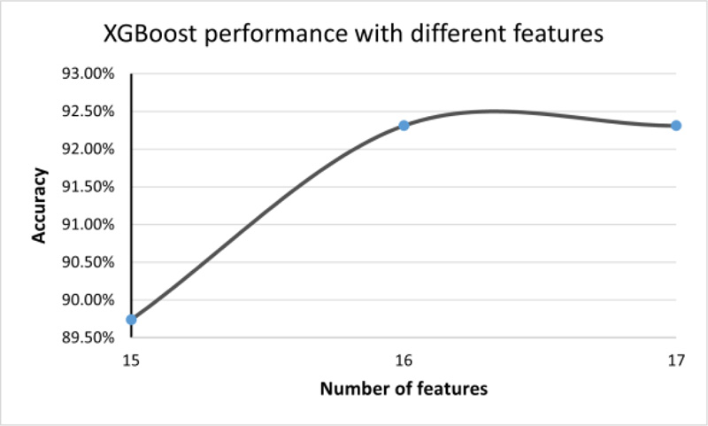
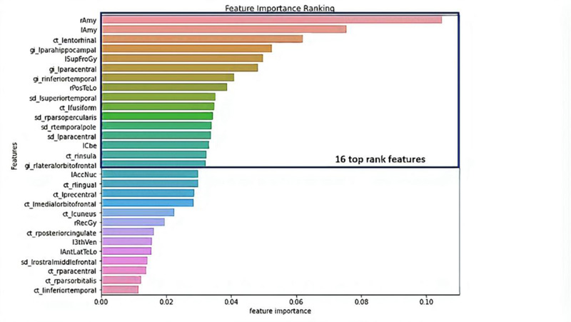
We got 16 top-ranked features: from the volume features group: rAmy, lAmy, lSupFroGy, rPosTeLo, and lCbe; from the gyrification index features group: lparahippocampal, lparacentral, rinferiortemporal, rparsopercularis, and rlateralorbitofrontal; from the sulcal depth features group: lsuperiortemporal, lparacentral, and rtemporalpole; and cortical thickness: lentorhinal, lfusiform, and rinsula, as illustrated in Table 3 and Fig. (5).
| Group | Features | Description |
|---|---|---|
| Volume | rAmy lAmy lSupFroGy rPosTeLo lCbe |
Right Amygdala Left Amygdala Left Superior Frontal Gyrus Right Posterior Temporal Lobe Left Cerebellum |
| Gyrification Index | lparahippocampal lparacentral rinferiortemporal rparsopercularis rlateralorbitofrontal |
Left Para hippocampal Left paracentral Right Inferior Temporal Right Pars opercularis Right Lateral Orbitofrontal |
| Sulcal Depth | lsuperiortemporal lparacentral rtemporalpole |
Left Superior Temporal Left paracentral Right Temporal Pole |
| Cortical Thickness | lentorhinal lfusiform rinsula |
Left Entorhinal Left Fusiform Right Insula |
Subsequently, these features were trained using three classifiers: SVM, KNN, and XGBoost. We considered four commonly used metrics which are ACC (accuracy), SEN (sensitivity), SPE (specificity), and AUC (area under the curve), to evaluate the classification performance. To achieve more stable results and maintain the same distance for all classifiers, we used 10-fold cross-validation to compare all methods: sensitivity = recall = 
Where TP, TN, FP, and FN are true positive, true negative, false positive and false negative, respectively. Area Under the Curve (AUC) is the two-dimensional area under the receiver operating characteristic (ROC) curve, which is a graph between the precision (y-axis) and recall (x-axis) at various thresholds (0-1).
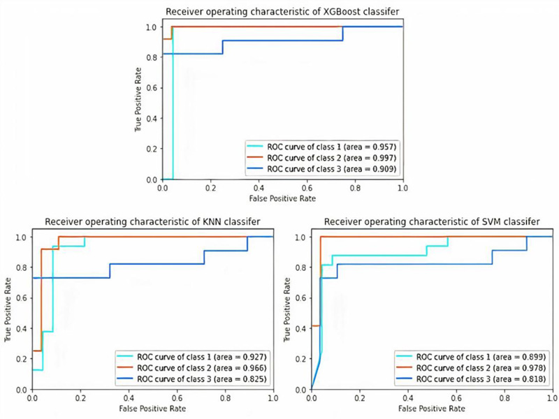
From Table 4, XGBoost gave the highest accuracy, which was 92.31%, among the other classifiers (SVM and KNN) with 89.18%. In addition, XGBoost has the best values for all metrics (precision, recall, F1-score, and AUC) over the SVM and KNN. It had the precision of 0.92, recall of 0.92, F1-score of 0.92, and AUC of 0.9543, as shown in Table 5 and Fig. (6).
| Classifiers | Accuracy |
|---|---|
| XGBoost | 92.31% |
| SVM | 89.18%, |
| KNN | 89.18%, |
| Classifiers | Stages | Precision | Recall | F1 score | AUCROC |
|---|---|---|---|---|---|
| XGBoost | AD | 0.94 | 0.94 | 0.94 | 0.957 |
| MCI | 0.92 | 1 | 0.96 | 0.997 | |
| NC | 0.9 | 0.82 | 0.86 | 0.909 | |
| Average | 0.92 | 0.92 | 0.92 | 0.9543 | |
| SVM | AD | 0.93 | 0.88 | 0.9 | 0.899 |
| MCI | 0.92 | 1 | 0.96 | 0.978 | |
| NC | 0.82 | 0.82 | 0,82 | 0.818 | |
| average | 0.89 | 0.9 | 0.893 | 0.898 | |
| KNN | AD | 0.88 | 0.94 | 0.91 | 0.927 |
| MCI | 0.86 | 1 | 0.92 | 0.966 | |
| NC | 1 | 0.73 | 0.84 | 0.825 | |
| Average | 0.913 | 0.89 | 0.89 | 0.906 |
The F1-score and AUC for the MCI stage had the highest values across all three classifiers, which means that with these selected features, we can differentiate the MCI stage from the others (NC and AD) in an excellent manner. Moreover, the AD stage had a quite high F1-score and AUC.
NC was the lowest stage in the F1-score among the other stages in all classifiers and had a quite high precision value and which means that all classifiers, in their errors, tended to classify NC as an AD or MCI patient. This status in disease diagnosis is preferable to classifying a patient as normal.
We used the original number of features for each group, and from Table 6, we can determine that volume features are the best group of features for detecting AD, followed by GI and CT groups. From the results, the SD feature group alone was not very effective in the diagnosis, although it improved the overall accuracy when combined with other feature groups.
| Classifiers | Volume (71) | GI (68) | SD (68) | CT (68) | Combined (275) |
|---|---|---|---|---|---|
| XGBoost | 82.05% | 66.67% | 58.97% | 66.67% | 71.79% |
| SVM | 69.23% | 64.1% | 46.15% | 66.67% | 82.05% |
| KNN | 79.49% | 66.67% | 51.28% | 69.23% | 79.49% |
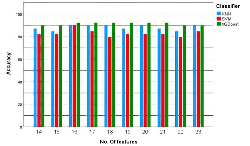
In Fig. (7), we performed the training and testing process for the three models (SVM, KNN and XGBoost) multiple times with different numbers of features (14-23 features). Therefore, XGBoost has the highest accuracy with the least number of features (16 features).
4. DISCUSSION
Recent research has reported using multivariable data analysis to classify dementia stages such as MCI and AD, as well as employing machine learning to predict dementia stages. Multivariate analysis studies have found that MCI is characterized by major temporal lobe atrophy, particularly in the superior and inferior temporal gyrus and hippocampus. The same study that classified early MCI in elderly healthy ageing people using only two structural regions in both hemispheres, the amygdala and hippocampus, found the best accuracy of up to 0.9 [43]. Temporal lobes are mostly associated with the encoding of memory and the processing of auditory information. The temporal lobe is also thought to play a critical role in processing certain aspects of vision and language [44]. Posterior medial temporal deterioration is related to disturbances in episodic memory in patients with AD [45].
Moreover, there is a study that reported that even in the early stages of dementia, the level of amygdala atrophy was associated with the severity of cognitive impairment (as determined by the MMSE and CDR-SB) [16]. In addition, amygdala atrophy is associated with abnormal motor behavior with a potential association with agitation and anxiety [46], which appear in Alzheimer’s. As it Plays a vital role in the memorizing and processing of emotional responses [47]. The mean volume of the amygdala is 3.17 cm3 lower than AD, which has 2.729 cm2 average volume [48].
Another study reported that the insular cortex, entorhinal, and fusiform were included with the most significant ROIs to predict a specific score for AD neuropathologic changes [49]. According to post-mortem AD neuropathological examination, entorhinal cortical thickness assessment was significantly related to neurofibrillary tangles in a recent pre-mortem MRI analysis [24]. Insular functions vary from basic functions, such as interoception and gustation, to integrative functions, such as decision-making, self-awareness, and self-consciousness [50]. Alzheimer's disease (AD) often involves visceral dysfunction and behavioral dyscontrol, which are not found in other disorders that affect cognition. This may be associated with autonomic instability and loss of self-awareness, and pathological changes within the insula cortex may play an important role [51].
On the other hand, the hippocampus and entorhinal cortex are critical for memory and spatial navigation [52]. The entorhinal cortex sends information to the hippocampus from different areas of the cerebral cortex, collectively known as the association cortex, while also returning processed information by the hippocampus back out to the association cortex [53]. These are the first brain regions to be affected in Alzheimer's disease. The average hippocampus volume for 66.27 ± 6.1 years is 5.202 (±0.76) cm3 and is reduced by 25% in Alzheimer’s [54]. The entorhinal cortex has an average volume of 1.93 cm3 for NC and 1.417 cm3 for AD [55].
Sulci have only been used in a few studies to distinguish between MCI and NC subjects. Among them, Park and his colleagues employed cortical thickness and sulcal depth to classify AD and MCI [56, 57]. Sulcal abnormalities have been associated with normal ageing and cognitive impairment in research [58, 59]. There is a consensus between most of the features reported in previous studies that are correlated with either MCI or AD, and the features that we employed in our model.
Our approach has the advantage of using a combination of features (volume, CT, GI, and SD) rather than depending on one group of features. As, they complemented each other and covered all the anatomical changes in AD. Besides, it classifies multiple stages of AD in one step and produces excellent results.
There is currently no predictive imaging biomarker for Alzheimer's disease that has confirmed/substantial neuropathologic correlations, especially in the early stage. However, employing the improvement in imaging and machine learning in the early detection of anatomical abnormalities in the prodromal stage, before they become clinically manifest, will be beneficial for preventing disease progression and designing effective treatments. By implementing XGBoost for the selected 16 features of the four groups of MRI images, the classification of NC, MCI, and AD can be performed with an accuracy of 92.31%.
CONCLUSION
In the proposed method, we achieved good performance for early-stage AD (MCI) detection, which is the most targeted stage to be identified. Moreover, we investigated the most reliable features for the diagnosis of AD.
This approach relies on using an embedded method such as XGBoost to extract the most important features representing AD from a large pool of features. In addition, three classifiers (XGBoost, SVM, and KNN) were used to determine the classifier with the highest accuracy. According to all the tested models, XGBoost was the most precise classifier because it had the highest precision, sensitivity, F-score, ROC-AUC, and overall accuracy of 92.31%. Moreover, the following features: rAmy, lAmy, lSupFroGy, rPosTeLo, lCbe, from gyrification index features group: lparahippocampal, lparacentral, rinferiortemporal, rparsopercularis, rlateralorbitofrontal, from sulcal depth features group: lsuperiortemporal, lparacentral, rtemporalpole, from cortical thickness features group: lentorhinal, lfusiform, rinsula are the most important features to detect MCI and AD together with NC. Furthermore, combining the volume features with cortical thickness, sulcal depth, and gyrification index of the brain regions yields more accurate results than using either of them independently.
LIST OF ABBREVIATIONS
| AD | = Alzheimer’s disease |
| MCI | = Mild Cognitive Impairment |
| NC | = Normal Aging Control |
| ADNI | = Alzheimer’s Disease Neuroimaging Initiative Database |
| MRI | = Magnetic Resonance Images |
| ROIs | = Regions Of Interest |
| KNN | = K-nearest Neighborhood |
| SVM | = Support Vector Machine |
ETHICS APPROVAL AND CONSENT TO PARTICIPATE
Not applicable.
HUMAN AND ANIMAL RIGHTS
Not applicable.
CONSENT FOR PUBLICATION
Not applicable.
STANDARDS OF REPORTING
STROBE guidelines were followed.
AVAILABILITY OF DATA AND MATERIALS
The data supporting the findings of this study are available within the article.
FUNDING
None.
CONFLICT OF INTEREST
The authors declare no conflict of interest, financial or otherwise.
ACKNOWLEDGEMENTS
Data used in this study was acquired from the Alzheimer's Disease Neuroimaging Initiative (ADNI) database (adni.loni.usc.edu). As such, the investigators within the ADNI contributed to the design and implementation of ADNI and/or provided data but did not participate in the analysis or writing of this paper. Data collection and sharing for this project were funded by the Alzheimer's Disease Neuroimaging Initiative (ADNI) (National Institutes of Health Grant U01 AG024904) and DOD ADNI (Department of Defense award number W81XWH-12-2-0012). ADNI is funded by the National Institute on Aging, the National Institute of Biomedical Imaging and Bioengineering, and through generous contributions from the following: AbbVie, Alzheimer's Association; Alzheimer's Drug Discovery Foundation; Araclon Biotech; BioClinica, Inc.; Biogen; Bristol-Myers Squibb Company; CereSpir, Inc.; Cogstate; Eisai Inc.; Elan Pharmaceuticals, Inc.; Eli Lilly and Company; EuroImmun; F. Hoffmann-La Roche Ltd and its affiliated companies Genentech, Inc.; Fujirebio; GE Healthcare; IXICO Ltd.;Janssen Alzheimer Immunotherapy Research & Development, LLC.; Johnson & Johnson Pharmaceutical Research & Development LLC.; Lumosity; Lundbeck; Merck & Co., Inc.;Meso Scale Diagnostics, LLC.; NeuroRx Research; Neurotrack Technologies; Novartis Pharmaceuticals Corporation; Pfizer Inc.; Piramal Imaging; Servier; Takeda Pharmaceutical Company; and Transition Therapeutics. The Canadian Institutes of Health Research is providing funds to support ADNI clinical sites in Canada. Private sector contributions are facilitated by the Foundation for the National Institutes of Health (www.fnih.org). The grantee organization is the Northern California Institute for Research and Education, and the study is coordinated by the Alzheimer's Therapeutic Research Institute at the University of Southern California. ADNI data are disseminated by the Laboratory for Neuro Imaging at the University of Southern California.
Names and indices of cortical regions in DKT40.
| Regions (Left Hemisphere) | Regions (Right Hemisphere) |
|---|---|
| 1 L_bankssts | 2 R_bankssts_right |
| 3 L_Caudalanteriorcingulate | 4 R_Caudalanteriorcingulate |
| 5 L_Caudalmiddlefrontal | 6 R_Caudalmiddlefrontal |
| 7 L_cuneus | 8 R_cuneus |
| 9 L_entorhinal | 10 R_entorhinal |
| 11 L_fusiform, | 12 R_fusiform |
| 13 L_inferiorparietal | 14 R_inferiorparietal |
| 15 L_inferiortemporal | 16 R_inferiortemporal |
| 17 L_isthmuscingulate | 18 R_isthmuscingulate |
| 19 L_lateraloccipital | 20 R_lateraloccipital |
| 21 L_lateralorbitofrontal | 22 R_lateralorbitofrontal |
| 23 L_lingual | 24 R_lingual |
| 25 L_medialorbitofrontal | 26 R_medialorbitofrontal |
| 27 L_middletemporal | 28 R_middletemporal, |
| 29 L_parahippocampal | 30 R_parahippocampal |
| 31 L_paracentral | 32 R_paracentral |
| 33 L_parsopercularis | 34 R_parsopercularis |
| 35 L_parsorbitalis | 36 R_parsorbitalis |
| 37 L_parstriangularis | 38 R_parstriangularis |
| 39 L_pericalcarine | 40 R_pericalcarine |
| 41 L_postcentral | 42 R_postcentral |
| 43 L_posteriorcingulate | 44 R_posteriorcingulate |
| 45 L_precentral | 46 R_precentral |
| 47 L_precuneus | 48 R_precuneus |
| 49 L_rostralanteriorcingulate | 50 R_rostralanteriorcingulate |
| 51 L_rostralmiddlefrontal | 52 R_rostralmiddlefrontal |
| 53 L_superiorfrontal | 54 R_superiorfrontal |
| 55 L_superiorparietal | 56 R_superiorparietal |
| 57 L_superiortemporal | 58 R_superiortemporal |
| 59 L_supramarginal | 60 R_supramarginal |
| 61 L_frontalpole | 62 R_frontalpole |
| 63 L_temporalpole, | 64 R_temporalpole |
| 65 L_transversetemporal | 66 R_transversetemporal |
| 67 L_insula | 68 R_insula |
| Regions (Left Hemisphere) | Regions (Right Hemisphere) |
|---|---|
| 1 L_Hip | 2 R_Hip |
| 3 L_Amy | 4 R_Amy |
| 5 L_AntMedTeLo | 6 R_AntMedTeLo |
| 7 L_AntLatTeLo | 8 R_AntLatTeLo |
| 9 L_Amb+ParHipGy | 10 R_rAmb+ParHipGy |
| 11 L_SupTemGy | 12 R_SupTemGy |
| 13 L_InfMidTemGy | 14 R_InfMidTemGy |
| 15 L_FusGy | 16 R_FusGy |
| 17 L_Cbe | 18 R_Cbe |
| 19 L_Bst | 20 R_Bst |
| 21 L_Ins | 22 R_Ins |
| 23 L_LatOcLo | 24 R_LatOcLo |
| 25 L_AntCinGy | 26 R_AntCinGy |
| 27 L_PosCinGy | 28 R_PosCinGy |
| 29 L_MidFroGy | 30 R_MidFroGy |
| 31 L_PosTeLo | 32 R_PosTeLo |
| 33 L_InfLatPaLo | 34 R_InfLatPaLo |
| 35 L_CauNuc | 36 R_CauNuc |
| 37 L_AccNuc | 38 R_AccNuc |
| 39 L_Put | 40 R_Put |
| 41 L_Tha | 42 R_Tha |
| 43 L_Pal | 44 R_Pal |
| 45 L_CC | 46 R_CC |
| 47 L_LatTemVen | 48 R_LatTemVen |
| 49 L_3thVen | 50 R_3thVen |
| 51 L_PrcGy | 52 R_PrcGy |
| 53 L_RecGy | 54 R_RecGy |
| 55 L_OrbFroGy | 56 R_OrbFroGy |
| 57 L_InfFroGy | 58 R_InfFroGy |
| 59 L_SupFroGy | 60 R_SupFroGy |
| 61 L_PoCGy | 62 R_PoCGy |
| 63 L_SupParGy | 64 R_SupParGy |
| 65 L_LinGy | 66R_LinGy |
| 67 L_Cun | 68 R_Cun |
| 69 CSF | 70 GM |
| 71 WM |